A problem of TCP Vegas

A duality model : Internet Congestion Control By Network Utility Maximization

reference : http://netlab.caltech.edu/assets/publications/Low-200203-vegas.pdf

Vegas model abstract

the objective of Vegas is to maximize aggregate source utility subject to capacity constraints of network resources
the Vegas algorithm is a dual method to solve the maximization problem

Preliminaries

A network of routers is modeled by a set \(L\) of unidirectional links with transmission capacity \(c_l\) , \(l \in L\) . It is shared by a set \(S\) of sources. A source s traverses a subset \(L(s) \subseteq L\) of links to the destination, and attains a utility \(U_s(x_s)\) when it transmits at rate \(x_s\) . For each link \(l\) , let \(S(l) = \{s \in S \| l \in L(s)\}\) be the set of sources that uses link \(l\) . By definition \(l \in L(s)\) if and only if \(s \in S(l)\) .

Objective of Vegas

the primal problem is:

\[\max _{x \geq 0} \sum_{s} U_{s}\left(x_{s}\right) \tag{1}\] \[\text { subject to } \sum_{s \in S(l)} x_{s} \leq c_{l}, \quad l \in L \tag{2}\]

where \(U_{s}\left(x_{s}\right)=\log x_{s}\)

If given routing matrix \(R_{ls}\) (1 if flow from source \(s\) uses link \(l\) , 0 otherwise), \(\sum_{s \in S(l)} x_{s} = Rx\)

Proof. By the Karush-Kuhn-Tuckertheorem a feasible source rate vector \(x^* \geq 0\) is optimal if and only if there exists a vector \(p^* = (p_l^* , l \in L) \geq 0\) such that, for all s, \(U_{s}^{\prime}\left(x_{s}^{*}\right)=\sum_{l \in L(s)} p_{l}^{*} \tag{3}\)

and, for all \(l\) , \(p^∗_l = 0\) if the aggregate source rate at link \(l\) is strictly less than the capacity \(\sum_{s \in S(l)} x^*_s < c_l\) (complementary slackness).

Dual Problem

Associated with each link \(l\) is a dual variable \(p_l\) . Define the Lagrangian of (1-2) as:

\[\begin{aligned} L(x, p) &=\sum_{s} U_{s}\left(x_{s}\right)+\sum_{l} p_{l}\left(c_{l} - \sum_{s \in S(l)} x_{s}\right) \\ &=\sum_{s}\left(U_{s}\left(x_{s}\right)-x_{s} \sum_{l \in L(s)} p_{l}\right)+\sum_{l} p_{l} c_{l} \end{aligned}\]

The objective function of the dual problem of (1-2) is \(D(p):=\sup _{x \geq 0} L(x, p)\)

Hence the dual problem is to choose the dual vector \(p=\left(p_{l}, l \in L\right)\) so as to

\[\min _{p \geq 0} D(p):=\sum_{s}\left(\sup _ {x_s \geq 0} \left(U_{s}\left(x_{s}\right)-x_{s} \sum_{l \in L(s)} p_{l}\right)\right)+\sum_{l} p_{l} c_{l} \tag{4}\] \[\text { subject to } p_l \geq 0 \tag{5}\]

Therefore, we can use iterative gradient projection algorithm to solve the dual problem

\[p(t+1)=[p(t)-\alpha \nabla D(p(t))]^{+} \tag{6}\]

Here \(\alpha\) is a constant stepsize, \([z]^{+}=\max \{0, z\}\) . The structure of the dual problem allows a decentralized and distributed implementation of the above algorithm.

When we want to solve \(\sup _ {x_s \geq 0} \left(U_{s}\left(x_{s}\right)-x_{s} \sum_{l \in L(s)} p_{l}\right)\) , it’s easy to get \(x^*_s=\frac{1}{\sum_{l \in L(s)} p_l}\)

We have \(D(p_l):= \sum_{s}\left(U_{s}(x_{s}^*)\right)-\sum_{s}\left(x_{s}^* \sum_{l \in L(s)} p_{l}\right)+ p_{l} c_{l}\)

So \(\nabla D(p_l(t)) = c_l - \sum_{s \in S(l)} x_s^*=c_l - \sum_{s \in S(l)} \frac{1}{\sum_{l \in L(s)} p_l}\)

So (6) can be rewritten as

\[p_l(t+1)=\left[p_l(t)-\alpha \left(c_l - \sum_{s \in S(l)} \frac{1}{\sum_{l \in L(s)} p_l} \right)\right]^{+} \tag{7}\]

Example

Consider the small network shown in the figure with two sources \(S_1\) and \(S_2\) that send TCP/IP packets to the destination D using the TCP Vegas protocol. The positive values for the edges represent the link capacities in Mbps. Each source transmits with rate \(x_i\) ≥ 0 (i = 1, 2). Formulate a network utility maximization using the logarithm utility function ( \(U_i = log(x_i)\) ) for each source and solve it using both CVX and the dual-based algorithm.

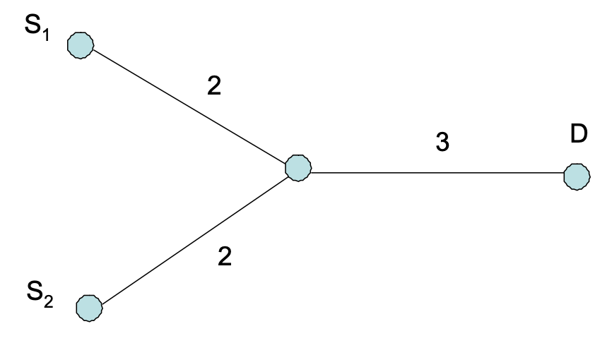
We have \(S=\{s1,s2\}\) \(L=\{l1, l2, l3\}\) \(L(s1) = \{l1, l3\}\) \(L(s2) = \{l2, l3\}\)

\(S(l1)=\{s1\}\) \(S(l2)=\{s2\}\) \(S(l3)=\{s1, s2\}\) \(c_{l1}=2, c_{l2}=2, c_{l3}=3\)

\(R= \left[ \begin{array}{cc} 1 & 0 \\ 0 & 1 \\ 1 & 1 \end{array} \right]\) \(x = \left[ \begin{array}{c} x1 \\ x2 \end{array} \right]\) \(p = \left[ \begin{array}{c} p1 \\ p2 \\p3 \end{array} \right]\)

According to (7), we have

\[\begin{aligned} p_{l1}(t+1) &=\left[p_{l1}(t)-\alpha \left(c_{l1} - \sum_{s \in S(l1)} \frac{1}{\sum_{l \in L(s)} p_l} \right)\right]^{+}\\ &=\left[p_{l1}(t)-\alpha \left(c_{l1} - \frac{1}{\sum_{l \in L(s1)} p_l} \right)\right]^{+}\\ &=\left[p_{l1}(t)-\alpha \left(c_{l1} - \frac{1}{p_{l1}+p_{l3}} \right)\right]^{+} \end{aligned}\]

likewise

\[p_{l2}(t+1)=\left[p_{l2}(t)-\alpha \left(c_{l2} - \frac{1}{p_{l2}+p_{l3}} \right)\right]^{+}\] \[p_{l3}(t+1)=\left[p_{l3}(t)-\alpha \left(c_{l3} - \frac{1}{p_{l1}+p_{l3}} -\frac{1}{p_{l2}+p_{l3}} \right)\right]^{+}\]

Now we can compute them separately see code2. However, we can also write them into matrix form and compute at once see code3.

We need to know \(\sum_{l \in L(s)} p_l = R^T p\) , \(\sum_{s \in S(l)} \frac{1}{\sum_{l \in L(s)} p_l} = \frac{R}{R^T p}\) , so

\[p(t+1)=\left[p(t)-\alpha \left(c - \frac{R}{R^Tp} \right)\right]^{+}\]

And finally \(x^*_s=\frac{1}{\sum_{l \in L(s)} p_l}\) , that is \(x1 = \frac{1}{p1+p3}\) , \(x2 = \frac{1}{p2+p3}\)

Code

code1

# using direct CVX
import cvxpy as cp
import numpy as np

x = cp.Variable(2)
c = np.array([2, 2, 3])
R = np.array([[1, 0], [0, 1], [1, 1]])
obj = cp.Maximize(cp.sum(cp.log(x)))
constraints = [x >= 0, R @ x <= c]
prob = cp.Problem(obj, constraints)
prob.solve()

print(f'optimal value is: {x.value}')

>>> optimal value is: [1.5 1.5]

code2

# using dual-based algorithm

p = np.array([0.1,0.1,0.6])

while 1:
  alpha = 0.1
  term = p
  p[0] = max(0, p[0] - alpha * (c[0] - 1/(p[0] + p[2])))
  p[1] = max(0, p[1] - alpha * (c[1] - 1/(p[1] + p[2])))
  p[2] = max(0, p[2] - alpha * (c[2] - 1/(p[0] + p[2]) - 1/(p[1] + p[2])))

  if sum(abs(term - p) ** 2) <= 0.01:
    break

print(f'optimal value is: {1/ (p @ R)}')

>>> optimal value is: [1.52912621 1.52912621]

code3

# using dual-based algorithm

p = np.array([0.1,0.1,0.6])

while 1:
  alpha = 0.1
  term = p
  p = np.maximum(0, p - alpha * (c - R @ (1 / (p @ R))))

  if sum(abs(term - p) ** 2) <= 0.01:
    break

print(f'optimal value is: {1/ (p @ R)}')

>>> optimal value is: [1.59090909 1.59090909]